Last time I posted on the crossover design I was hoping to be able to design the woofer-mid and mid-tweeter sections separately. As is most commonly the way with passive electronic filter design, that wasn’t possible because the phase shifts the woofer-mid crossover introduces affects the way in which the tweeter and mid range add together, meaning it must be taken into account to obtain a flattish response. Also, I failed to take into account the effect of the phase compensation network on the woofer-mid crossover, which will also change the phase relationships and ruin our previous attempt at the design.
Therefore the most appropriate way to deal with the problem is to deal with it as a complete system and optimise the crossover for a flat response. This we can again do with the nlminb() minimiser in R, all we need to is define an appropriate cost function to minimize.
As with the previous attempt at a crossover design for the woofer-mid region, the proposal is to have a first order high pass filter for the mid-range, which when combined with the response of the driver gives a nominally 3rd order acoustic response, and a complimentary 3rd order low pass section for the woofer. At the mid-tweeter crossover we propose having a third order low pass for the mid-range and a complimentary 3rd order high pass for the tweeter. These parts of the crossover all go into the cost function and parameters to optimise.
Originally I had also added the mid-range box volume as a parameter to optimize and although it converged to a good result it chose a mid-range box volume of 15 litres, which is simply too large, firstly because such a large mid-range driver volume is impractical, and secondly because such a large volume adds little additional stiffness to the mid-range meaning that the acoustic power handling will be compromised. We want a reasonably small mid-range box volume to add stiffness to the driver, thereby raising the level of power it can handle before the cone gets driven into the non-linear region. I chose a compromise box volume of 5 litres and fixed it at that in the design, then let the optimizer take care of the rest.
Phase Compensation
As mentioned in an earlier post, phase compensation applied to the mid-range is required to compensate for the phase reversal in the tweeter as we pass through the resonant frequency of the driver. We could apply it to the tweeter instead of the mid-range but we will need to use bipolar electrolytic capacitors here and I would rather not have those in tweeter signal path to keep it as clean as distortion free as possible.
The graph below shows the theoretical phase difference between the mid-range and tweeter (the red plot) and the phase difference after phase compensation (the blue plot). Remember that this theoretical plot agrees well with observations found in the previous post.
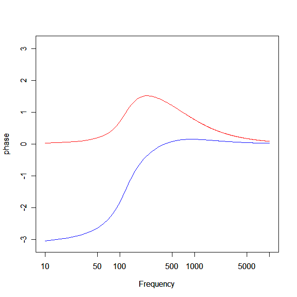
The phase compensation is achieved with a first order all-pass lattice network which is explained in the Wikipedia article found here. Remember the idea is to make the phase difference as near as possible to zero in the mid-tweeter crossover region (1kHz). This compensation achieves that down to a frequency of around 450Hz at which point it increases to a asymptotic phase lag of two pi radians. This should be good enough to ensure good crossover behaviour between the mid-range and tweeter. The components required in our case are an L of 3.05mH and a C of 82.1 uF assuming a load of 6.1 ohms (the voice coil resistance).
Optimised Crossover Response
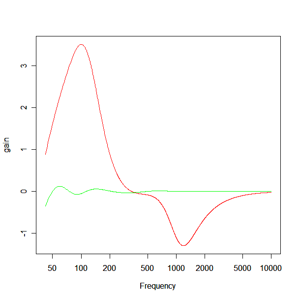
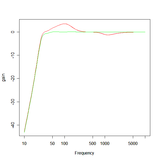
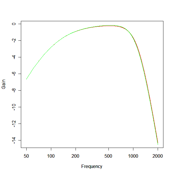
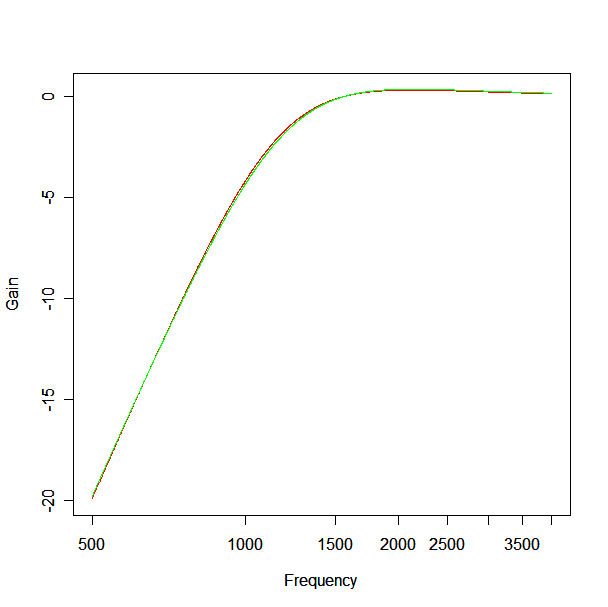
Using the optimiser to find the optimum crossover response and using a basic 3rd order Butterworth structure as the starting point, we find the responses shown below. The first zoomed in to the system pass band and the second showing the woofer roll off. The red plot shows the response of our starting point crossover and the green plot shows the optimised result. By running it through the optimiser we’ve taken a response deviation of +3.5, -1.2dB and reduced it to something more like +/- 0.1dB. All in all, a great improvement!
It doesn’t end here though, because the component values in the design are not the ones available (you can only buy components with a limited set of component values) and the inductors you can buy all have some series resistance. Therefore we need to add into the response the effect of series resistance in the inductors and only use available component values to synthesize the filters. This we do by using component values closest to the ideal, plotting the response of the ideal against the actual and then manually trying different real component combinations until we get a response that is as close to idea as possible.
In the case of the woofer, the model called for component values of 22.4mH, 5.49mH and 431uF. The actual component values that best fit are 22mH (series resistance 0.96 ohm), 5.6mH (series resistance 0.45 ohm) and 400uF. The comparative responses are shown below. The red plot is the ideal and the green plot is the actual response.
Note that there is significant deviation in the pass band which is due to the insertion loss of the filter owing to the high series resistance in the inductors. There is little that can be done about this without making the inductors impractically large and expensive. It’s just a fact of life that inductors operating at the low frequency end of the spectrum will generally have low Q’s leading to significant deviation from the ideal.
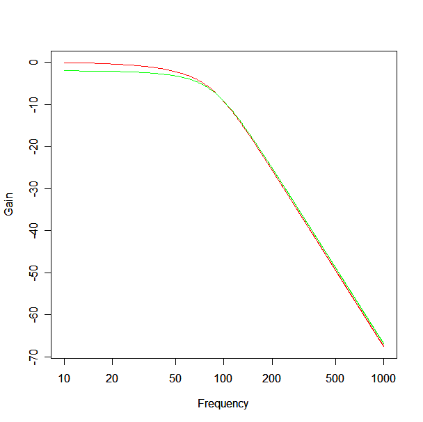
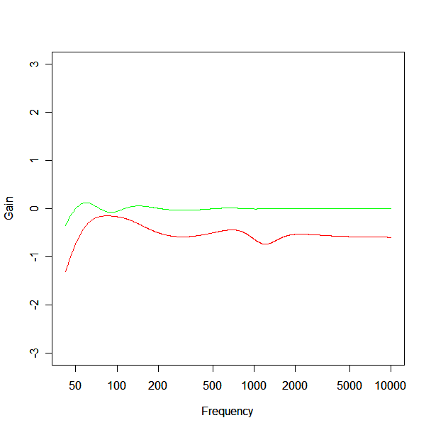
For the mid-range the comparison of ideal and actual is shown below. Here the agreement is much closer owing to the inductors operating at a higher frequency, thereby increasing the Q’s of the inductors (Q being the ratio of reactive to resistive impedance in the inductors).
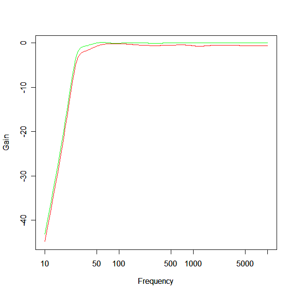
For the tweeter the comparison of ideal and actual is shown below. Again the agreement is pretty close though not as close as for the mid-range case. This is due to the sensitivity of the tweeter crossover filter (you can see it has a ringing second order pole pair by the peaking gain) to changes in component values.
Combining these actual responses we obtain the following combined responses as compared with the ideal combined responses. Here the green plot is the ideal and the red plot is response with actual component values. The actual response is not as flat but is within a +/- 0.5 dB envelope which is still pretty good.
The complete crossover design is shown below. It certainly isn’t simple but the added complexity of this design should provide real gains in performance over a simpler structure. Half the crossover complexity simply stems from the required impedance equalisers for each driver. However, it isn’t really an optional component. When using high order crossovers, any reactive impedance in the filter load will create nasty peaking or notching responses in the actual crossover behaviour, so it is absolutely necessary to provide impedance equalisation for the drivers.
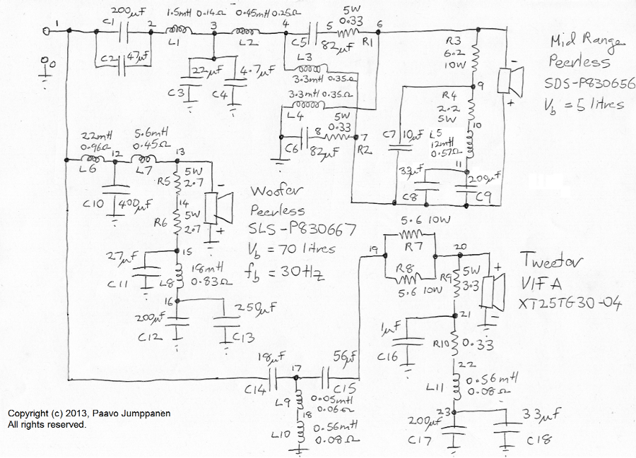
Also note that the mid-range and woofer are both wired anti-phase to the tweeter. This is a part of the phase equaliser for the mid-tweeter crossover point and must be adhered to. If you happen to wire them up the other way around you will get a horribly deep notch at the mid-tweeter crossover point.
Components C5,C6,L3,L4,R1 and R2 comprise the phase equaliser for the mid-range. The resistors R1 and R2 are included to compensate for the series resistance of the inductors L3 and L4. R3,R4,C7,C8,C9 and L5 form the impedance equaliser for the mid-range. C1,C2,C3,C4,L1 and L2 form the actual mid-range crossover filter circuit.
Components R5,R6,C11,C12,C13 and L8 form the impedance equaliser for the woofer. Remember from and earlier post that ideally this would have a second series resonator for the second peak in the driver impedance created by a bass-reflex enclosure, but we omit it because the components required for it are beyond what is available and too expensive to warrant the inclusion of it. L6,L7 and C10 form the actual 3rd order low pass filter for the woofer.
Components R9,R10,C16,C17,C18 and L11 form the impedance equaliser for the tweeter. R7 and R8 form an attenuator for the tweeter to bring its output in to line with the mid-range (the tweeter has a higher sensitivity than the other drivers). C14,C15,L9 and L10 form the actual 3rd order high pass filter. Note that you might think that we could do away with L9 and 0.56mH is pretty close to 0.61mH but owing to the sensitivity of the response to component values for that section, we must include it or otherwise include a significant deviation from the ideal response.
NGSPICE Circuit Simulation
As a final check on the performance of the crossover we introduce an NGSPICE circuit simulation for it to validate it. NGSPICE is a commonly used (in electrical engineering) circuit simulation program that dates back to the 60’s. Fortunately there is an online version available here if you are willing to put up with the advertising it shows you, or like me, use a browser that disables that page javascript so you are blissfully unaware of it.
So how does it work? It’s pretty simple to use. All you need to do is to create a network description of the circuit, define the type of analysis and request the results. To define the circuit network you label all the nodes in the circuit diagram with numbers, then define the components as being connected from one node to another and its value. By custom, the 0 node is assumed to be ground. If you take a look at the circuit diagram above you’ll note that I have already labelled all the nodes. The SPICE network that represents this circuit is shown below.
Complete crossover simulation
* Use to download raw simulation from https://www.ngspice.com
V1 1 0 AC 1

* Mid range crossover
C1 1 2 200u
C2 1 2 47u
L1 2 29 1.5m
RL1 29 3 0.14
C3 3 0 22u
C4 3 0 4.7u
L2 3 39 0.45m
RL2 39 4 0.25
* Mid range phase equaliser
C5 4 5 82u
L3 4 49 3.3m
RL3 49 7 0.35
R1 5 6 0.33
C6 0 8 82u
R2 8 7 0.33
L4 0 69 3.3m
Rl4 69 6 0.35
* Mid range impedance equaliser
C7 7 9 10u
C8 7 11 33u
C9 7 11 200u
L5 11 911 12m
RL5 911 10 0.57
R4 10 9 2.2
R3 9 6 6.2
* Mid range equivalent circuit
Rm1 6 200 6.1
Lm1 200 201 0.37m
Cm1 201 7 384.18u
Rm2 201 7 14.115
Lm2 201 7 7.3665m

* Woofer crossover
L6 1 91 22m
RL6 91 12 0.96
C10 12 0 400u
L7 12 912 5.6m
RL7 912 13 0.45
* Woofer impedance equaliser
R5 13 14 2.7
R6 14 15 2.7
C11 15 0 27u
RL8 15 915 0.83
L8 915 16 18m
C12 16 0 200u
C13 16 0 250u
* Woofer equivalent circuit
Rw1 13 100 5.5
Lw1 100 101 0.78m
Cw1 101 102 3927u
Rw2 101 102 10.390
Lw2 101 102 11.267m
Cw2 102 0 560.0u
Rw3 102 0 37.5289
Lw3 102 0 16.36m

* Tweeter crossover
C14 1 17 18u
RL9 17 917 0.06
L9 917 18 0.05m
RL10 18 918 0.08
L10 918 0 0.56m
C15 17 19 56u
* Attenuator
R7 19 20 5.6
R8 19 20 5.6
* Tweeter impedance equaliser
R9 20 21 3.3
C16 21 0 1u
R11 21 22 0.33
RL11 22 922 0.08
L11 922 23 0.56m
C17 23 0 200u
C18 23 0 33u
* Tweeter equivalent circuit
Rt1 20 300 3.0
Lt1 300 301 0.01m
Lt2 301 0 2.028m
Rt2 301 0 13.89
Ct1 301 0 65.71u

*.AC LIN 2048 0 22050Hz
*.END
.AC DEC 50 10 10000
.END
It is necessary to define an AC voltage source : V1 between nodes 1 and 0. For all the inductors which have a series resistance associated with them I’ve added a node not marked on the schematic to include it in the simulation. For example,
L1 2 29 1.5m
RL1 29 3 0.14
Shows an inductor of 1.5mH and series resistance 0.14 ohm connecting node 2 to node 3 with the unmarked node being 29.
Another point to note is that for the simulation to be correct we must include the actual impedance of the drivers in the simulation via equivalent circuits. For the mid range the impedance is realised through Rm1, Lm1, Cm1, Rm2 and Lm2, for the tweeter it is realised through Rt1, Lt1, Lt2, Rt2 and Ct1 and for the woofer it is realised through Rw1, Lw1, Cw1, Rw2, Lw2, Cw2, Rw3 and Lw3.
The other entry of note is the one that names the type of analysis we want SPICE to do which is,
.AC DEC 50 10 10000
This line say we want an AC analysis (small signal frequency response) with decadal frequency samples with 50 points per decade from 10Hz to 10kHz. Then all that is required is to tell SPICE what you would like to plot. This we do with,
db(v(6,7))
db(v(13))
db(v(20))
1.0 / abs(i(V1))
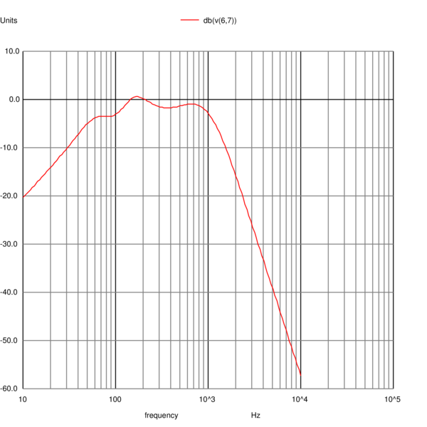
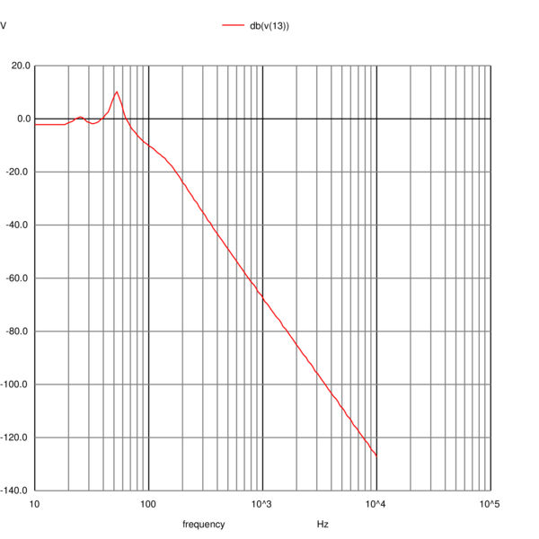
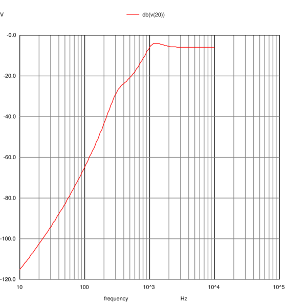
which asks for dB plots of the voltage between nodes 6 and 7 (the mid-range input), the voltage at node 13 (the woofer input) and the voltage at node 20 (the tweeter input). We also plot the inverse absolute output current of the voltage source which actually represents the input impedance of the crossover (remember V=IR and V=1 in this case).
If you copy and paste the network into the first edit field and the plots above into the second one and press the “simulate and plot” button, NGSPICE will compute the response of the crossover and return the following graphs.
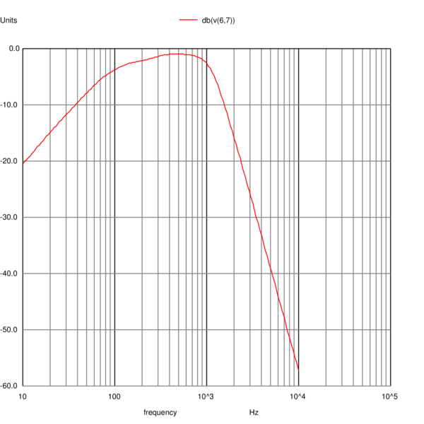
Mid-range Input
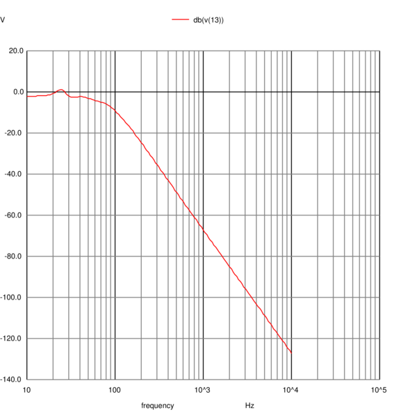
Woofer Input
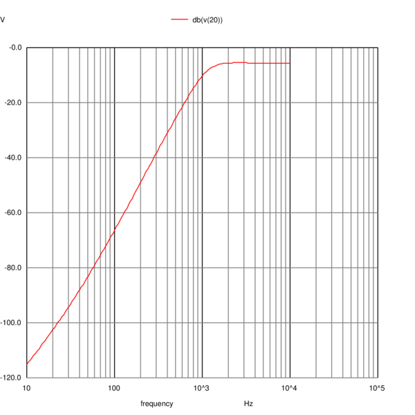
Tweeter Input
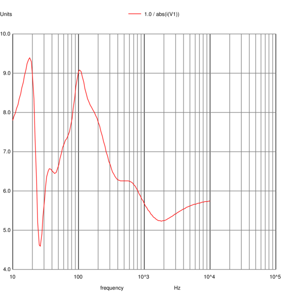
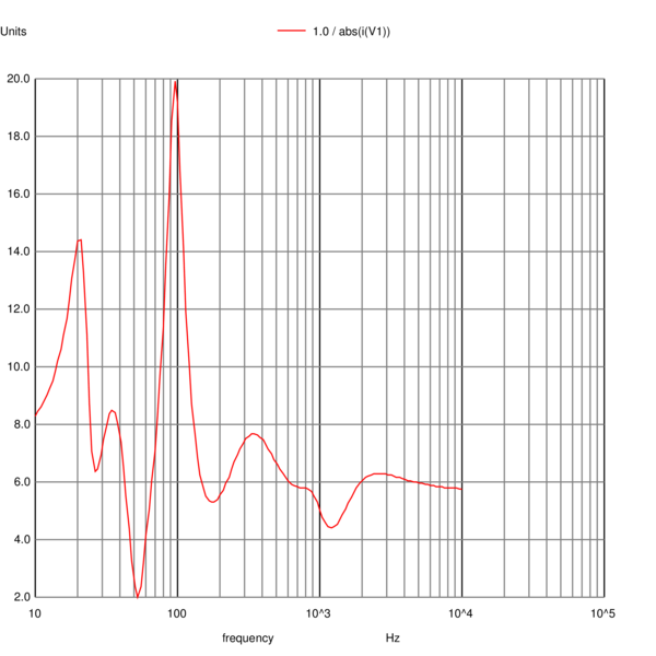
Crossover Input Impedance
The mid-range and tweeter inputs look the way we expect them too. The woofer input shows a slight peaking at 24Hz due to the impedance peak that was not equalised. The woofer impedance is nominally 6 ohms and being bound between 9.5 and 4.5 ohms. Certainly not resistive but the loudspeaker shouldn’t present any problems to any amplifier and you shouldn’t need exceptional speaker cables to use them.
With our SPICE simulation it is relatively easy to demonstrate the effect of omitting the impedance equalisers or at least the LRC component. All we need do is replace the R component with a large resistance making it appear open circuit. If we do so the resulting responses are,
Mid-range Input Without Equaliser
Woofer Input Without Equaliser
Tweeter Input Without Equaliser
Crossover Input Impedance Without Impedance Equaliser
Looking at the responses the importance of the equalisers is patently clear. The responses exhibit unwanted peaking around the resonances of the drivers. The input impedance of the crossover is also more reactive than the case of with driver impedance equalisation.
Final Simulation Results
As a final step we can integrate the SPICE simulation results back into our R model to obtain the modelled acoustic output of the loudspeaker system. If we do so we obtain the result below. The red plot shows the combined response, the green plot is the woofer output, the blue plot is the mid-range output and the orange plot the tweeter output.
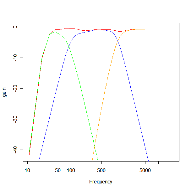
The response is not as flat as the simpler simulation and the difference most likely arises from the driver impedances not being perfectly equalised (perfect equalisation was assumed in the previous results). Even so, the response is within a 1dB envelope. It also extends to below 30Hz.
Power Handling and Resistor Power Ratings
To determine system power handling we need to assume a shape for the typical power spectral density of the signals a loudspeaker will be driven by. For this I’ve assumed a basic pink noise power spectrum with a 2nd order (12 dB per octave) roll-off below 30Hz and a gentle 3dB per octave roll off above 2kHz. Then the electrical rating of the loudspeaker system can be determined by the manufacturers power rating and the theoretical power proportion delivered to each driver assuming the described signal power spectral density. As it turns out, the limiting factor on power handling is the mid-range unit because it carries the majority of the signal power. The theoretical electrical power handling is 121 Watts.
The resistor power ratings are determined by using the SPICE simulation results to determine the voltage across each resistor based on the assumed power spectral density of the input signal (with a power of 121 Watts). The power dissipated in the resistor is then that voltage squared divided by the resistance. Then the nearest power rated resistors are chosen for the crossover. This is indicated on the crossover schematic.
All that remains is to design an enclosure to fit the design constraints : a box volume of 70 litres for the woofer, box frequency of 30Hz and a box volume of 5 litres for the mid-range. It is mostly an issue of finding a style and appearance you like rather than a highly technical design. This I’ll cover in my next post.