| Har-Bal Harmonic Balancer: An Introduction to Version 3 |
|
Har-Bal™ new thinking, new directions... Limitations and MotivationsThe first generation of Har-Bal introduced high resolution filtering coupled with spectrum analysis and a novel "loudness compensated" filter designing user interface to improve the capabilities of mastering engineers in tackling troublesome equalisation issues. As good as the fundamental design is it has shortcomings when dealing with certain classes of mastering problems. Non-stationary Tonal BalancePrior to the era of hyper-compression and hyper-limiting many recordings that presented tonal imbalance issues could satisfactorily be treated with static equalisation. That is, one EQ setting applied to an entire track. In the pursuit of absolute loudness new factors are introduced as a result of an interaction between compression/limiting and the track dynamics : the forte passages within tracks often have accentuation of the upper mid range as a side effect of dynamics processing leading to a harshness of tone in those passages. If treated with static equalisation the harshness can be counted but only at the expense of the tonality of the quieter passages that become coloured by the equalisation. With tracks of this nature what is required is equalisation that is taylored to specific parts of the track. The contemporary approach to "dynamic" equalisation issues is the application of multi-band compression to a track. This is a less than ideal approach for a number of reasons. Firstly, the application of equalisation through multi-band compression is a rather indirect approach to equalisation that is difficult to accurately target to a specific track. Secondly, attacking what is essentially an equalisation issue with compression necessarily alters the dynamics of a track because the "effective" equalisation is being constantly adjusted. Thirdly, because of the constant adjustment, processing artifacts from multi-band compression can occur. The Har-Bal approach to such equalisation issues is to instead split a track up into its structural components (intro, verse, chorus, verse, chorus, bridge etc.) and have a custom filter for each. Within each segment the filter characteristic is fix so the dynamics are essentially un-altered, only the relative dynamics between sections are altered. Because the filter characteristic is fixed there is no dynamic adjustment side effect except at the transition from one section to another. However, if the transition point is chosen carefully, significant change in equalisation without audible side effect is possible because the timbre of the track naturally changes from, say the verse to the chorus, and through our listening experience we expect to hear a corresponding change in timbre. The net effect is that the potential side effect of our change is masked in the track structure. With careful filter design artifact free dynamic equalisation is possible and the new user interface within Har-Bal 3 provides many aids to getting the design right. Channel Specific Issues and Problems in Stereo ImageSometimes a pre-master track has been inappropriately mixed and has imaging problems. Perhaps the track needs to be prepared for vinyl mastering and requires monophonic bass or perhaps some parts in the the track are panned too widely or too narrowly and for whatever reason re-mixing is not a possibility. Perhaps you would like to demonstrate to the mix engineer the imaging you believe the track requires so he/she can have something to reference against to achieve that end. Har-Bal 3 addresses these issues by providing seperate mid and side filtering capabilities coupled with full mid and side spectrum analysis. From this analysis the spread of the imaging can be readily seen from the relative strengths of the mid and side spectrums and readily altered by independent filtering applied only to the side component. For completeness, Har-Bal also provides independent left and right filtering to attack channel specific issues should the need arise. Defining a Coherent SpaceSometimes one is presented with a recording that lacks a sense of immediacy, of not being present in the performance because of a lack of recorded ambiance. Sometimes ambiance is present in some parts but completely absent in others (lead vocal for example), leading to a sense of disconnection between parts. To bring some cohesion to these types of issues Har-Bal 3 introduces Haas zone cross-coupled ambiance processing. This new Har-Bal Air implements an idealised ambiance tail with a reverberation time of less than 50 milliseconds (Haas zone) and less ambiance at higher frequencies to give a natural warthm to the ambiance. Being Haas zone ambiance, there is little coluration to the natural timbre of the recorded music except when used in the extreme. The new Har-Bal air simply provides a space, particularly when the space is absent in the recording. In mono recordings Har-Bal air can also be used to simulate stereo effectively and naturally. Controlling the Dynamic RangePre-masters of popular music usually have more dynamic range than is ideal for the genre. To obtain a commercially loud master some compression combined with limiting is usually required to achieve suitably high levels. For such pre-masters it was not generally possible to obtain suitably loud masters in Har-Bal alone because it had not means of reducing dynamic range except through limiting, which if used exclusively to obtain loudness often has delaterious side effects. To provide for such cases, Har-Bal now includes a means of altering the dynamic range through mapping the average track level to a different one. This approach is more closely comparable to volume riding than traditional compression and works by mapping the volume envelope obtained in analysis to a different one specified through a novel interface. This approach leads to a compressed sound that is quite unlike traditional compression.
The Inner Workings of Har-Bal 3Track AnalysisTo provide for the ability to perform dynamic filter and the mid and side processing a new approach to analysis is required. In traditional Har-Bal the analysis is an average for the entire track. In the latest generation we need support for track splitting with arbitrary split points that we cannot know a-priori. To cope with such a requirement in a timely fashion we need to store a partial analysis of instantaneous spectrum results over the entire track time so that we can quickly average them over a track segment to give the segment analysis result. This is achieved by taking overlapping time windows at nominally 50 millisecond intervals and obtaining a spectrum estimate through Fourier transformation, binning the result into 1/12 octave bins and storing the result to disk in an analysis file (file extension .hba). The spectrum estimate for a stereo track is actually four fold because we need analyses for mid (left + right), side (left - right), left and right components. We also record the average and peak power levels for each of those components per time step. This strategy is summarised in Figure 1 below. 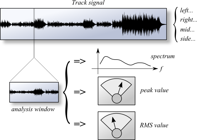
Figure 1: The comprehensive analysis scheme implemented within Har-BalThis degree of analysis has a number of side effects. Firstly, an analysis file must contain a lot of information because we record four spectrum estimates at each 50 millisecond interval for the entire track. Typically for a stereo PCM encoded wave file the corresponding analysis file (.hba) is larger than the original source. This is unavoidable if you want to have access to the power that this degree of analysis gives. Secondly, as a side effect of this detail, a real-time spectrum can be displayed in the Har-Bal analysis graph. Having access to this real-time information is invaluable in determining which parts of the spectrum are responsible for uncomfortable sounds in a given recording. Thirdly, the average power component for each 50 millisecond interval can be combined to form a time series that accurately represents the track volume envelope, which in turn can be used as a basis for implementing dynamic range processing. Filter StructureTo cater for the requirements of independent filtering of left, right, mid and side components and to provide Haas zone ambiance, a new filter structure is required. Figure 2 illustrates the new structure of the Har-Bal filter block. Keep in mind that each component of this filter can have many different response functions owing to track splitting (for each segment in a Har-Bal filter there is one of these filter blocks). 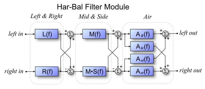
Figure 2: The basic Har-Bal filter module structureLeft and right filters come first, then after decoding to mid and side components, the mid and side filters follow. Note however, that the mid filter component is included in both the mid and side filters. This is deliberate by design. The reason being that the mid spectrum view is the view you will most often use to design equalisation schemes for tracks but when you apply equalisation in this view you do not want to alter the stereo image. For that to be guaranteed we must apply the same equalisation to the side component, hence its inclusion. However, the side component can be adjusted independently to allow us to alter the stereo image when we see fit to do so. 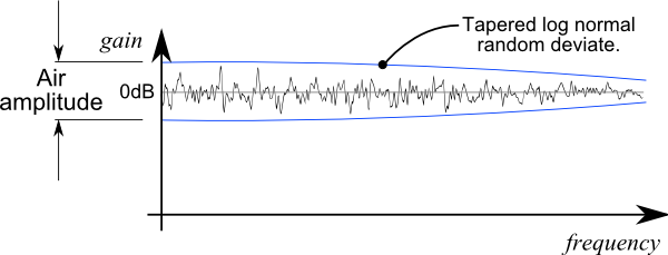
Figure 3: Frequency Domain Synthesis of Haas Zone AmbianceA flat frequency response is deviated by a log normal random deviate with characteristics suitable to confine the ambiance tail within the Haas zone. The magnitude of the deviate is controlled by the Air setting. To create a natural and pleasing sounding ambiance the magnitude of the deviate is tapered off at higher frequencies. This has the effect of making the reverberation time of low frequencies longer than that of high frequencies, a characteristic that is appropriate for music reproduction. This frequency domain representation is translated to the time domain by realising a minimum phase impulse response that matches the given frequency reponse. This results in a impulse response like that in Figure 4. 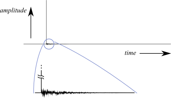
Figure 4: Resulting Time Domain Impulse response with Ambiance TailThis process is used to realise all four responses required to synthesise the complete Air filter network, except that the cross couple responses of Alr (f) and Arl (f) have no unit impulse component, just the ambiance tail. Each filter uses a unique uncorrelated random deviate in the synthesis process and it is this uniqueness of response which results in a spatialising effect. 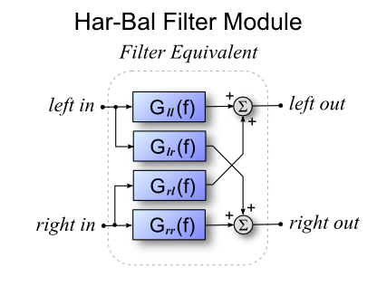
Figure 5: The basic filter module structure reduced to a structurally simpler equivalent to reduce signal processing demandsThe Har-Bal filter module (as illustrated in Figure 2) contains eight filters. If implemented independently, more processing power will be used than is actually necessary. As an efficiency measure, the entire filter structure is replaced by the equivalent filter shown in Figure 5 and only requires four filters per module. This compares favourably with the first Har-Bal implementation which only has two filters (left and right, but with a common response). What is Mid - Side Encoding?The Har-Bal filter module makes use of Mid - Side encoding and decoding to provide extra control in mastering equalisation. For those unfamiliar with it, Mid - Side encoding is defined by the following equations: Mid = Left + Right You can see that with a mono source Side = 0 as Left = Right. So the level of the Side component relative the Mid component gives an indication of the stereo spread of your mix. To reconstruct Left and Right from Mid and Side use the following equations: Left = (Mid + Side) / 2 It can be noted that if the Side component is reduced in amplitude relative to the Mid component we will narrow the stereo image. This can be inferred bt the fact that In the limit as the amplitude of the Side component is reduced to zero the mix tends to monophony. You can use this fact to alter the stereo image in Har-Bal by applying filtering to the side channel in a given Har-Bal filter module. Segmented FilteringTo obtain artifact free processing a track should, when necessary, be split into segments based on musical piece structure. Figure 6 shows a typical segmentation and how many filter responses are involved. In this case the track is split into eight segments and there are 9 filters : one for each segment plus one overarching filter for the entire track. Har-Bal provides this additional filter to make it easier to control the overall colour of the track. Without it, should you wish to change the overall colour you would have to clumsily apply the same filter response to each of the eight segments individually. 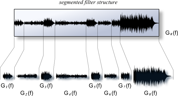
Figure 6: Building a hierarchical filter taylored to the track musical structureCreating, deleting, modifying and navigating the segments and corresponding filters is handled through the time-line control in Har-Bal. Filters are selectable through the selection bars on the timeline control as indicated in Figure 7. This schematic representation naturally represents the actual filter heirarchy whilst also allowing easy navigation of the heirachy. The two traces in the time line show the average and peak power time series obtained from the track analysis and the extent of the time shown corresponds to the selected filter, which in this case corresponds to the outermost overarching filter. 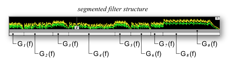
Figure 7: Representation of filter structure through the Har-Bal time lineFor each selected filter Har-Bal displays the peak and average spectrum traces with and without filtering from the top of the heirarchy downward, as in Figure 8. In this case, as the outermost (top) filter is currently selected, the average spectrum shows the estimated spectrum that results from the application of all the filters applied to their corresponding segments plus the effect of the overarching filter. If an individual segment were selected then the spectrum estimate would show only the average spectrum for the time range of that segment and the effect of that filter on that spectrum only. The reasoning here is that if you are adjusting a segment filter you only want to know the effect that the segment filter has on the segment average and not the effect of any filtering applied above the level of the segment. Hence, in this case the effect of the outermost filter is not included. 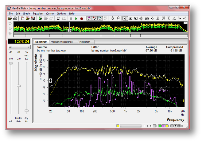
Figure 8: Har-Bal spectrum viewWith the frequency response view selected we see the filter response of the selected filter, which in this case is the outermost one (see Figure 9). Whichever is selected, Har-Bal only shows the response of the selected filter and not contributions from other levels of the heirarchy. The logic here being that for frequency response view we wish to see the filter response contribution for the selection. The frequency response view shows the change in level applied to the components of the spectrum at a particular frequency. It is analogous to the image cast by the sliders on a graphic equaliser and in this case shows a high pass response with a cut-off at 30Hz. 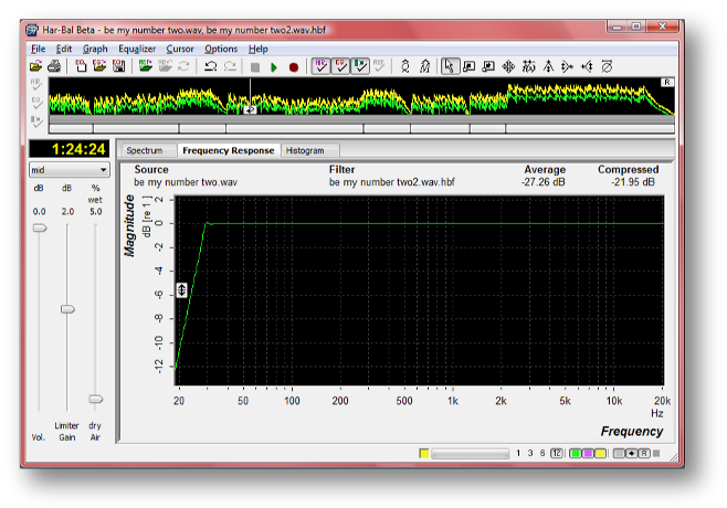
Figure 9: Har-Bal frequency response viewThe final view Har-Bal provides is the histogram view, which corresponds to the histogram of timeline levels, binned in 1 dB wide bins, both peak and average, for the selected segment. This view is also used to design a dynamics processing scheme for the selected segment using dynamics node editing. Figure 10 shows the histogram view for the entire track and the effect of a simple compression scheme on the histogram. 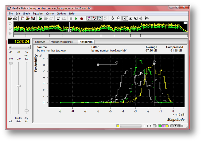
Figure 10: Har-Bal histogram response viewHistograms are used to quantify track dynamics because they provide a complete, convenient and quantitative snapshot of the track characteristics, unlike metering which can only ever show you a very localised snapshot. The histogram in Har-Bal is a graph representing the likelihood (probability) of the x- value (horizontal axis) occuring. In our case the horizontal axis is level in dB and it is binned in 1dB wide bins (hence the city line appearance of the graph). If you take any one of those tall rectangles, look at the dB value below it and the percent value corresponding to it's height, you can interpret it as follows. Lets say the column I'm looking at is centred on -5 dB and it's height is 7%. That is telling me that for 7% of the time the level is between -5.5dB and -4.5dB (note that the bin is 1dB wide and centred on -5dB). That could be either the peak level or the average level depending on whether you are looking at the green or the yellow trace. If you happen to move the gain slider you'll note that the histogram marches up and down the horizontal axis by the amount of gain you apply. Now that you know what the histogram is you should see why that should be: because a level that was in the range from -5.5dB to -4.5dB after a 2 dB gain will now be in the range of (-5.5 + 2) dB to (-4.5 + 2) dB. However, you might be wondering why when you increase the gain the 0dB bin gets taller and taller. Well, if you think about it, the maximum level we can produce is 0dB. If something was in a -3dB bin and we apply a 6dB gain it can't go into the +3dB bin because there isn't one. What actually happens is the limiter cuts in and forces it into the 0dB bin. Thus, the more you push the gain higher the more the topmost bin in the histogram fills up as the values from other bins are forced into it. This is a very useful thing in mastering because you can immediately see how over-zealous your limiting is. As an example, take any current generation master of popular music and look at the histogram of the peak level and you will almost certainly see a massive 0dB bin and little left in the other bins. That is what over-limiting does to the dynamics of your track. It squashes them into oblivion. Dynamics ProcessingThe dynamics processing in Har-Bal is based entirely on the average level envelope that you see in the time-line. You create a transfer function to map the input average level to a new output average level and Har-Bal uses it to figure out what gain to apply dynamically prior to the limiter at any point in time. Unlike conventional dynamics processing, it doesn't use attack - decay envelope extraction. The envelope it already has from the analysis. As such the gain change that tracks the music is in sync and symetrical about the content. By that I mean with a normal compressor you would typically have a fast attack time and slow release which means that the gain quickly drops at the start of a transient and slowly rises at the tail after the transient. Now you'll probably think that makes no sense and will sound aweful. However it doesn't sound aweful, and here is the reason why. In traditional compression we principally have fast attack and slow release because a compressor cannot predict the future so it doesn't know when to pull down the level and if it does it slowly a very big transient will push through before it has a chance to bring it down. We have a slow release time because fast gain change will lead to a lot of distortion. Because Har-Bal knows the entire history of the track we don't need fast attack because we know when to pull the level down. The net result is that the dynamics processing in Har-Bal works more like the volume riding technique of recording engineers of days gone past where they would adjust down the level while the music is being recorded because they knew when the loud parts were comming. This point is clearly illustrated in Figure 11, which shows the difference between envelope detection used traditionally and in Har-Bal. 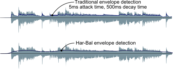
Figure 11: A comparision of envelope detection in tradional and Har-Bal dynamics processingBy using a slow moving envelope for dynamics processing we ensure that the short term transient material remains largely unaltered and we simply change the relativity between loud and soft passages of a track. This also ensures that very little distortion is introduced by dynamics processing. These two factors are responsible for the clean sound of Har-Bal's dynamics processing. How do you actually use it. Well, as hinted at before you design an input-output transfer function using the dynamics node editing tool in the histogram view. Why the histogram view? Because the histogram view shows you a summary of the dynamics content and to stick with a theme in Har-Bal, it will show you the effect your dynamics processing has on that histogram. The process works like this. A transfer characteristic is made up of nodes. You create a node by clicking the dynamics node tool anywhere on the histogram graph. The node displays as two circles connected by lines, one filled and one not. Think of the unfilled one as an "O" for output. It represents the level you are mapping the input to. The filled circle represents the input level. So a typical compression scheme would work like this. You look at the average level histrogram (green trace) and look at the highest level it has (ie. where the hill comes down to the flat on the right hand side). At that point you put a node with input and output equal. Why? because we want the top of the histogram to stay put and just squash up the the bottom (quieter) parts. Its saying map the input level to the output level of, for arguments sake lets say it is -15dB. Now look at the other side of the hill. Where the left hand slope comes down to the flat we want to map that level to a higher level (compressing it) so we press down the left mouse button (that sets the input level) then drag it up to the level we want to map it to and release the mouse button (that is the output level). For example, it might be and input of -60dB and an output of -45dB. You'll note that after releasing the mouse Har-Bal gives you an updated histogram showing the effect of the scheme on it and also the updated average track level figure of merit. You'll also note that if you happen to render those changes and re-analyse the result the prediction is pretty accurate. Figure 12 illustrates this example. The upper node mapping input level to output level is place at -15dB and is at the upper most limit of the un-processed histogram (the black trace). The lower node maps the input level from -60dB to -45dB, the light grey trace shows the effect of the dynamics processing on the track histogram and the processed level shows the average track level after dynamics processing. In this case we see the level has gone from -27.26dB (un-processed) to -21.95dB (processed). 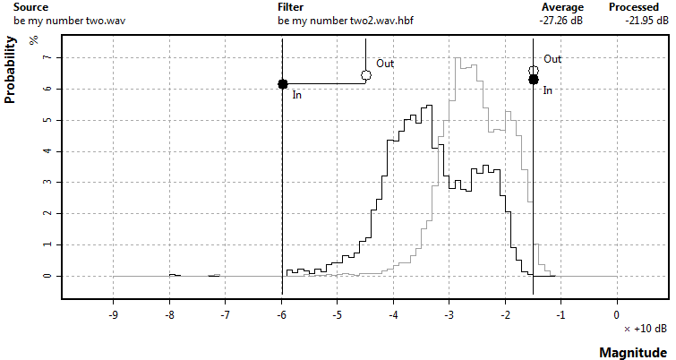
Figure 12: A compression processing exampleIf you are used to looking at compression in terms of transfer characteristics mapping input to output level and compression slopes, we can relate Har-Bal's histogram views and nodes to just that. This relationship is illustrated in Figure 13. The histogram on the left is obtained by transforming or projecting it through the input - output transfer characteristic (the solid dark line). When adjusting the output node you'll notice that the status line in Har-Bal displays information about the left and right slopes. These figures correspond to the transfer characteristic line slopes as indicated. Figure 13: Relationship between the Transfer Characteristics and Dynamics Processing NodesA couple of observations can be made regarding histograms. When compressing, the width of the histogram is compressed but that squeezing makes the peak higher. This occurs because the area under the curve is constant and sums to 100% (ie. everything). You can think of it as a lump of plasticine you use to model a hill. If you squeeze the sides together then the plasticince pushes out at the top because the volume has to go somewhere. Similarly, if you stretch it, then it falls down (ie. dynamic range expansion). Another thing to note is that this processing can be used for more than just compression. Another useful thing to use it for is noise gating. What I would typically do for that application is to provide a split at the end of the track where it fades away and apply dynamics processing to that split to gate the noise. The setting of the nodes is essentially exactly the same as with compression except you now map the input to a lower level on the left hand side to make the noise quieter. If you have additional dynamics processing applied to the overall track the two mappings are combined. It all makes for a powerful and flexible architecture for managing the dynamic range of your track. Example FiltersThe best way to illustrate the power of the approach that Har-Bal 3 allows is through hearing the results obtained from well designed filters. This process is inherently objective and the resulting sound is heavily influenced by the interpretation an expectation of the person constructing the filter. As such I would like to point out at the outset that these filters are a product of my personal expectations for the tracks in question. What I have done you may or may not agree with, though that is beside the point. Rather, In listening to and assessing the example filters given, I suggest that you adjust your mindset from "which version sounds best" to "how much can we transparently change the sound of a track through filtering in Har-Bal without damaging its integrity". In particular, you should pay attention to the filter transitions from segment to segment and try and pick them through listening alone. That is, without watching the timeline cursor during playback. Also note that most of the filters have a degree of gain cut applied globally to ensure that what you are hearing is not overly coloured by limiting upon limiting. The examples given are deliberately commercial releases to avoid the criticism of the examples being contrived and not "real world" cases. They have already been mastered by professional engineers of some standing though I shall resist from naming them. Should you wish to know the necessary information should be discoverable on the net. Finally, as they are commercial releases they must be paid for, so if you would like to hear how the filters perform you will need to part with a minor sum of money to the music download site of your choice, though if you choose to download from a location other than the links provided below, be aware that you may have chosen a different mastering to the one I have used to design the filter. By downloading from the location given below you are guaranteed to be hearing what I hear.
More on Understanding HistogramsA histogram shows the frequency (as in how often something occurs) of an event. It comes from probability and statistics theory. For a pure statistics explanation, lets say I have a bag of ping-pong balls with numbers written on them. The numbers are in the range of 1 to 10. Some of the numbers are the same. Lets say you empty them out and you see these numbers: 1,3,4,5,3,3,1,4,6,7,9,9,9,9,10,7. A histogram showing the frequency of the numbers is constructed by counting how often each number occurs. So in the above case we have,
That is, there are two 1's, no 2's, three 3's, two 4's, one 5 and so on and so on. A normalised histogram usually specifies things in percentages so to convert into a percentage we divide by the total number of balls in the set and multiply by 100. The frequency numbers therefore become, 100 * (2 / 16), 100 * (0 / 16), 100 * (3 / 16), .... because there are 16 balls in the set. That is what a histogram is. You may note that for normalised histograms the sum of all the frequencies is always 100% because that is the set of all balls in the bag. Now in the context of Har-Bal's histogram, the balls are each of the sample points on the time line (which are spaced at a nominally 50ms interval) and the number on the balls is the average value for the average histogram and the peak value for the peak histogram. The main difference with the above example is that the time line is a real number (ie. fractional) so how do you group them. Well we group them in "bins" of 1dB width. What does that mean? Take a small subset of average values: -0.3dB, -0.4dB, -0.7dB, -1.6dB, -2.4dB .... The bins are centred on exact dB values of 0dB,-1dB,-2dB,-3dB .... The boundary from one bin to the next is the mid-point between centres. The top bin 0dB is special because it doesn't have an upper boundary.
Going back to the sequence of average values, all we do is figure out which bin the number fits into and when we find that bin we add 1 to it because this corresponds to a count of 1 value fitting in that bin. -0.3dB fits in the 0dB bin, so does -0.4dB, -0.7dB fits into the -1dB bin, -1.6dB fits into the -2dB bin, -2.4dB fits into the -2dB bin and so on and so on. After counting all the values in the bins they are normalised by converting to percentages (100 times the bin count / total number of time line samples). A histogram, like an average spectrum is much more useful for judging the dynamics of a track because it presents it in a static single image summary. Show me a histogram of the time line and I can tell you immediately whether it has high or low dynamic range, what the limits of the dynamic range are, whether it has a bi-modal behaviour (as in loud parts and quiet parts), whether it has been over limited and so on and so on. It is all there to be seen in the histogram. If you find it hard to believe just open up a track you know to have high dynamic range and a track you know to have low dynamic range. Compare the histograms. Can you see the difference? The pattern is obvious and immediately revealing. The histogram also contains within it the total average level within it. If you give me the histogram I can calculate the track average from the data it presents. It makes a great deal of mathematical sense to summarise dynamics with histograms. Why is Har-Bal 3 slower at updating filters?If you are a Har-Bal 2.3 user used to playing a track real-time and making and hearing Har-Bal filter changes in near real time you'll probably be wondering why Har-Bal 3 is so slow at updating. Well, it isn't because the code is slower but rather, what it has to realise is much greater. The detailed answer is as follows. Har-Bal 2.3 realises only left and right filters with a common response (ie ganged). In the basic Har-Bal 3 filter block Har-Bal realises four filters. It has two extra responses to realise : the new Haas zone ambiance derived "air" which uses cross-couple filters. That is the first two fold factor difference but there is more. To keep CPU usage during playback to a minimum Har-Bal uses an equivalent filter to realise the independent left, right, mid, side and air filters. By doing so, we reduce the complexity by half but it means that all those responses are lumped together, which consequently also means that if you want to have real-time switchable air and eq (toggle air, toggle eq) then we have to calculate four different combination's of filter responses, three that are non-trivial. That is,
no air + no eq, trivial So now we have a 6 fold increase in the amount of calculation to realise Har-Bal 3 filters over Har-Bal 2.3. In the future that will increase further because a proposed feature is additional room compensation equalisation in Har-Bal 3. It's already coded for but there is no front end to add or indeed design the responses. With room EQ it then becomes,
no air + no eq + no room eq, trivial So with that version it will grow to be a 14 fold increase in the amount of calculation required. Given the added amount of calculation you'll probably be asking what's the point. The point is that with the more powerful analysis and the more powerful filtering, Har-Bal 3 can improve on tracks with relative ease that Har-Bal 2.3 can never make headway on. I know that with certainty from experience with using it. There is so much stuff around today that Har-Bal 2.3 just can't help with a great deal, especially when hyper-compression is involved. For me personally, despite the slower speed at realising filters, I feel absolutely no desire to go back and use version 2.3 and if I'm forced to 2.3 I'm always looking for the Har-Bal 3 features it can't do and despairing. The near real time filter update in Har-Bal 2.3 is neither here or there to me. It is entirely in-consequential. If it is critical to you I can't offer a solution because there isn't one, bar not offering all the added processing power of Har-Bal 3 which is something retro-grade and of no value to me. Real-time filter updates isn't even in the design use case as far as I'm concerned so the lack of it doesn't rate as a fault because it is not a design goal. If that is what you need and can't live without you'll either have to stick with Har-Bal 2.3 for as long as it will continue to work on current generation machines, or go with the myriad of other EQ tools you can find in plugin format, or as dedicated hardware units. What is important in the Har-Bal design is the mid /side filtering capability, the track splitting and near instantaneous update to spectrum averages based on whatever your filters do, the dynamics processing and the predictive average level estimates, real-time spectrum, complex time selection and filtering to control rogue resonances (when that feature is implemented), room eq compensation (when that feature is implemented), improved air that even works on mono sources, playable track referencing to allow you to easily bring consistent sound to compilations and all the other aids Har-Bal provides. I don't use Har-Bal in a realtime fashion, not even Har-Bal 2.3. Rarely have and I dare say, rarely will. That mode of operation has no value to me. If it were that important to me I can do what I pretty much always do, which is to do spectrum editing with nothing playing, then play and toggle EQ to hear the difference. Sound better, keep it, sound worse, undo it. It isn't a usability issue for me. Not having the power to do everything else that Har-Bal 3 offers is. There are a few other points that should be mentioned regarding this version and it's speed. It is not compatible with older machines and by older machines I mean ones more that four years old. The reason being that current generation intel processors do floating point faster than fixed point so all the signal processing in Har-Bal 3 is now in floating point. Older machines are slower on floating point than fixed point so when run on an older machine Har-Bal 3 will seem very slow. Fast disk access is a necessity for Har-Bal 3 because it needs to read and write a lot of information to files to support the real-time spectrum and track splitting. As such, you should never open a file on an external drive, be that a network drive or a thumb drive. Doing so will almost certainly result in very slow response. |