| Har-Bal Harmonic Balancer |
|
Har-Bal™ new thinking, new directions... Har-Bal TutorialsHar-Bal is the software that introduces the concept of Harmonic Balancing and the means of achieving it. In this section we introduce the software and the process of Harmonic Balancing as implemented through Har-Bal. Before continuing and further, I thoroughly recommend that you first read the Har-Bal introduction as you will learn a great deal about the structure of the software, its capabilities and the thinking behind its implementation. Har-Bal Layout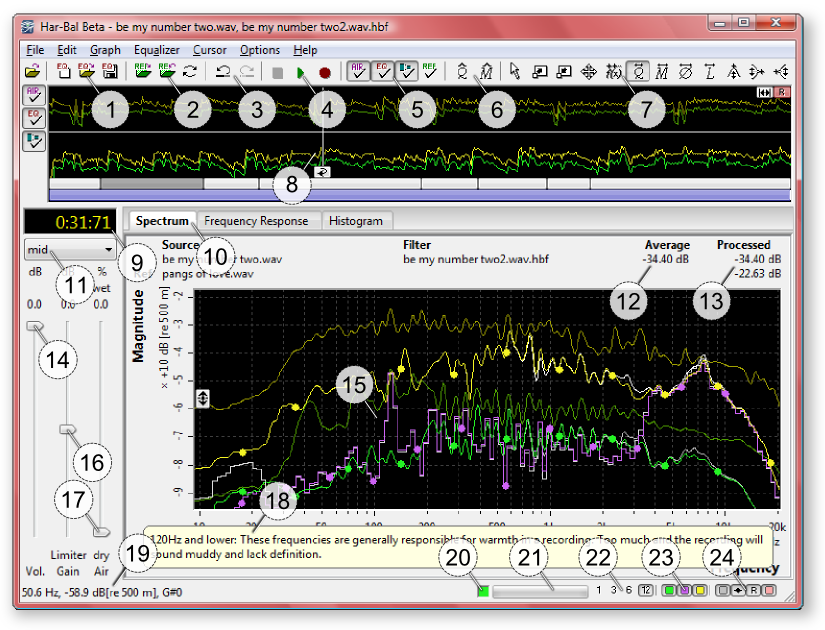
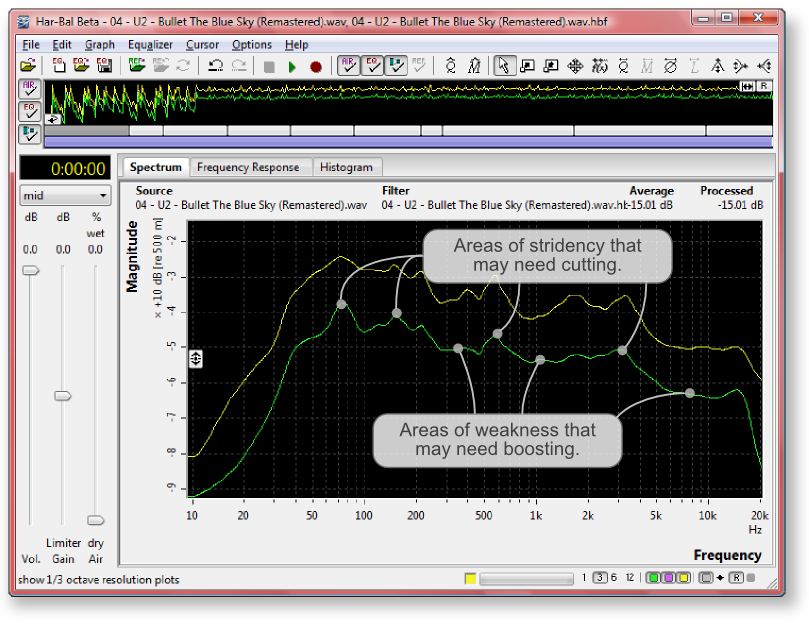
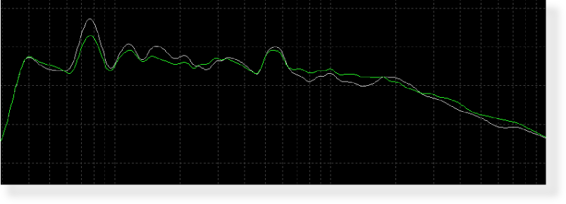
1. Filter related toolbar buttons 2. Reference related toolbar buttons 3. Filter design undo/redo toolbar buttons 4. Playback/Record control related toolbar buttons 5. HB Air, Filter, Dynamics and Reference control toolbar buttons 6. IntuitQ and IntuitMatch toolbar buttons 7. Filter editing and view control toolbar buttons 8. Time line control 9. Time display 10. View Selection Tab 11. Spectrum selection dropdown list 12. Average power figure of merit indicator 13. Processed figure of merit indicator 14. Volume control slider 15. Spectrum view 16 Limiter gain control slider 17. HB Air control slider 18. Tips popup 19. Status bar message area 20. Cursor focus indicator 21. Limiter gain reduction meter 22. Spectrum resolution buttons 23. Spectrum view toggle buttons 24. Spectrum view control buttons Where to Start?Har-Bal works with sound files only, so a good place to start is with collecting the source material to harmonically balance. For a list of supported file types consult the Open Command topic. It is recommended that source material should be arranged such that each track in a given compilation is in a separate file. You could, if you wish, perform harmonic balancing on a single file corresponding to an entire album but the outcomes that will result is likely to be less than optimal. This is because each track in a compilation has its own specific characteristics, which when lumped together, become lost in the whole. Given a set of tracks that you wish to master we are now ready to start. The first thing to do is to open one of your tracks using the Open Command. The first time you do this on any given track Har-Bal will proceed to analyse the spectrum content. This may take some time depending upon the length of the track and the speed of your computer but once done the result is saved to disk for re-use. If you then re-open the same track, provided it has not been modified in any way, Har-Bal will open it immediately by reading the analysis file of the track created on first opening it. Alternatively, if you have a compilation of many tracks that you are going to work on, you can pre-analyze those tracks in the background while you work on another file in Har-Bal by using the File | Batch Analysis menu command. For the sake of this tutorial I shall be demonstrating Harmonic Balancing of a selection of tracks from the U2 album, The Joshua Tree. Beginning a SessionAssuming that you are mastering new material or re-mastering old material then the first thing you should do is thoroughly listen to the compilation of tracks to build a mental picture of the sound the producers are trying to achieve. Make note, mental or otherwise, of anything that concerns you. After doing so pick the track from the compilation that has a broad spectrum (typically tracks with the most instruments and instruments that are played loudly) but also the best sound quality. The reason for this choice is that the first track we master will become a reference for the remaining tracks. If you were to chose a slow song it won't fill the entire spectrum and then you will have some difficulty drawing inferences from your reference if you were to then open a busy track. Using the Open Command I open track 4, Bullet the Blue Sky as the first track as it has a full spectrum and a reasonable balance. When the analysis runs to completion the spectrum view shows the following result. 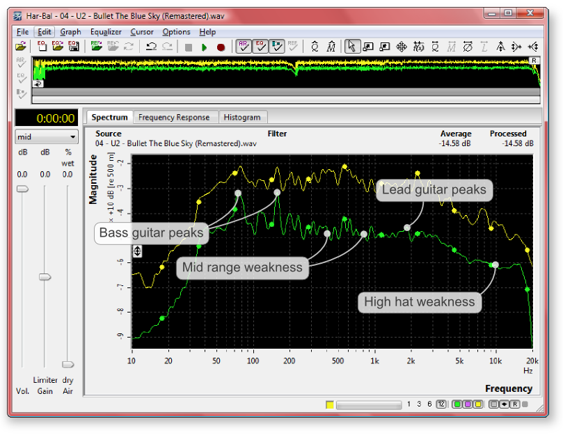
Figure 1: Mid-spectrum view of "Bullet the Blue Sky"The spectrum display has three traces; the lower trace is the average energy content of the track at different frequencies, the top trace is the peak energy content of the track and the violet trace shows the real-time spectrum content. On listening to the whole track the following observations are apparent. The track has a prominant bass guitar part that has a boxy character. Whilst the drum part is a prominant part of the track, the high hat sounds as though it is suffering from distructive interference arising from leakage of the high hat sound into other microphones on the drum kit (perhaps the overheads). The snare drum, though prominent, also sounds a tad wooden, lacking a sense of crispness. The lead guitar is largely well controlled but has occasional stridency in the upper mid-range (2 - 3kHz). Finally the lead vocal sounds brittle in places, though generally well controlled. Looking at the spectrum we see that it extends from around 40Hz to 18kHz. There are two prominant peaks at around 75Hz and 150Hz corresponding to the bass guitar part, which are most likely responsible for the box character of the part. The region between 4 - 14kHz is somewhat subdued and corresponds to the weakness in the high hat part. There is possibly some weakness in the mid range area in places. Rather than attempt to address these issues in this view we should instead split the track along song structure lines to obtain a better understanding of the sources of the imbalances and a better corrective filter for the track. Splitting the track into its parts (intro, verse, chorus, verse, etc.) is achieved with the split shortcut command applied to dragging the time line cue point. I find a useful what of identifying the correct point to split at is to first zoom into the region where a transition from one part to the next occurs. To zoom mouse over the timeline, press the left mouse button down and drag the highlight over the region of interest. 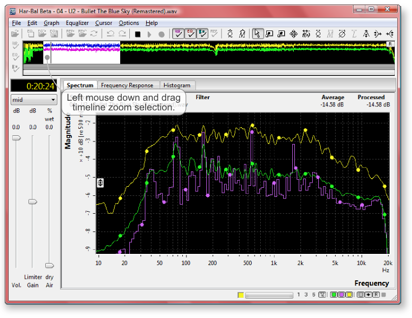
Figure 2: Zooming in to the time line of "Bullet the Blue Sky"I find the best way to create a split is to zoom in to a close region either side of the transition point and set the track playing close to the point of transition from one part to the next. Then watch the time line track cursor and listen for the transition. When you think you know the general region where it occurs, then press down the left mouse button on that point and release it to resume playback from that point. If the location is correct you will hear the entire beginning of the section cleanly and if you chose wrong then it will sound discontinuous. If the latter move you location in the direction appropriate and try again until you have found the transition point. At that stage press and hold the left mouse button down on that position in the time line and press Ctrl+S to create the split point. This process is illustrated in Figure 3. 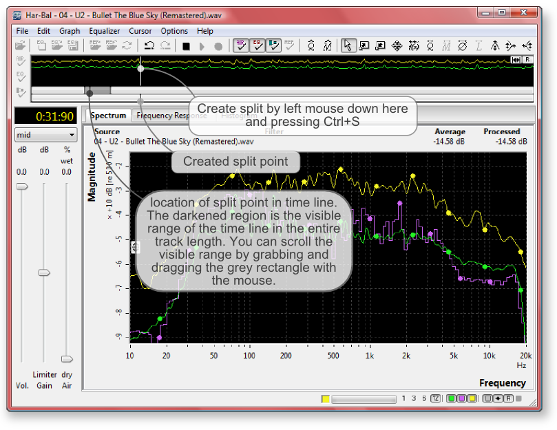
Figure 3: Creating split pointsTo avoid loosing work it is useful to occasionally save changes to a Har-Bal filter file. Selecting the File | Filter | Save Command, we save it to the file "04 - U2 - Bullet The Blue Sky (Remastered).wav.hbf". Then we continue on adding split points to the track time line. We add 9 split points at the times outlined in Table 1.
Table 1: Split Point TimesHaving created the track segmenting we can now begin constructing an equalisation scheme for the track. Start by selecting the first segment. This is done by mousing over the first segment and clicking it with a left mouse button press. 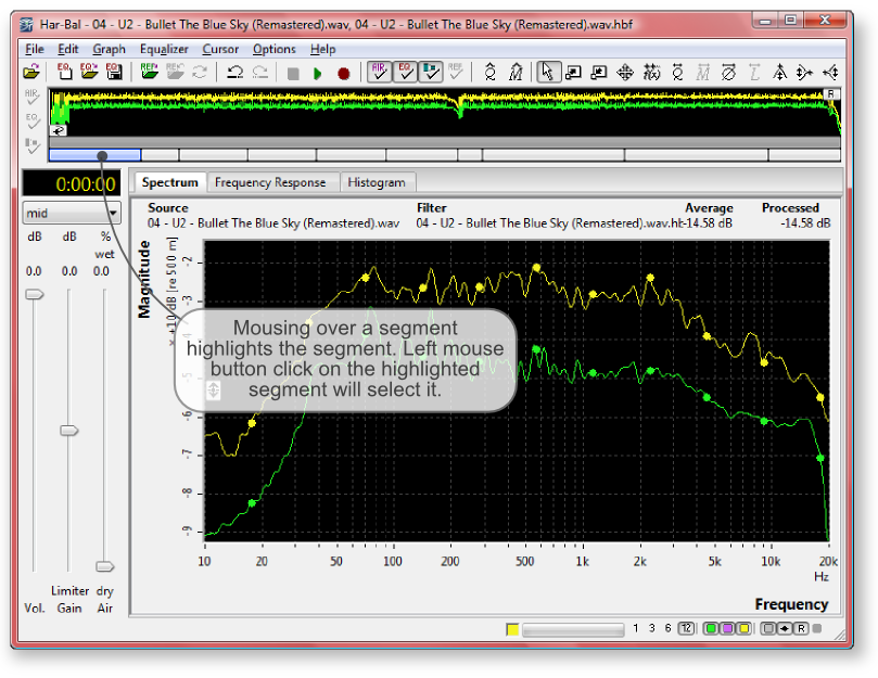
Figure 4: "Bullet the Blue Sky" track segmentation : selecting the first segmentBefore continuing on with the design of the equalisation scheme for this track we need to introduce and discuss the technique of empathetic equalisation. Empathic Equalisation : What is it and why does it work?Empathetic Equalisation can be loosely defined as the process of high Q notching and peaking applied to the tracks average spectrum (in the 1/12th octave resolution view) in such a way as to produce a uniform average spectrum when viewed with 1/3rd octave resolution. It isn't a rigid prescription but rather, a recommended approach that needs to be tempered by what you hear. If a particular edit produces detrimental results then undo it, re-assess your approach and try a different variation.
Rule 1:
Rule 2:
Rule 3:
Rule 4:
Rule 5: 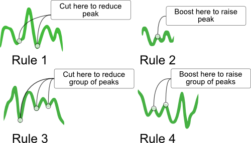
Figure 5: Rules 1 - 4 of the Empathetic Equalisation techniqueSo why use these rules? Is there any deeper reasoning as to why we should equalise using this approach? In fact, there is justifiable reasoning behind it. The general consensus you are likely to hear elsewhere is that you should only use low Q boosting and cutting and usually with only a small degree of boost or cut, yet we are suggesting essentially the complete opposite of the widely held view. Why so? If you happen to look at the structure of musical notes played on typical instruments you will generally find that each played note (or percussive hit for that matter) is composed of a short lived transient component that generally has a broad spectrum and a much longer lived resonant component that is largely confined to a handful of frequencies, the harmonics as it were. This is clearly illustrated with a sonargraph of a single note plucked on a guitar string as shown in Figure 6. It is clearly visible that immediately after the string pluck a broad range of frequencies are generated but the high frequency components quickly die away to leave us with the long lived harmonics. Indeed, the initial broad band spectrum is essentially atonal and corresponds to the spectrum content of the impulsive event, in this case the act of plucking, giving rise to the string vibration. The components that live on are the ones that resonate in the guitar string. 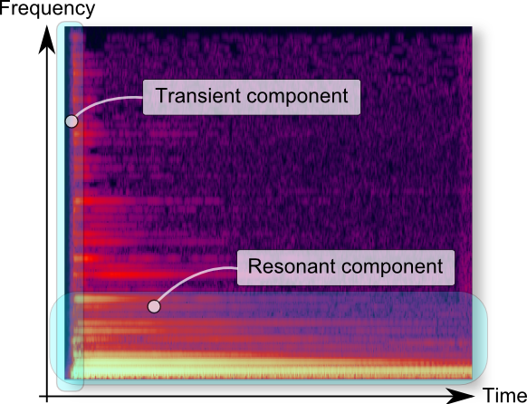
Figure 6: Sonargraph of a plucked guitar string. Brighter colours correspond to higher spectrum magnitude. Note that the transient component of the sound covers the entire frequency range and is short lived, whilst the resonant component is long lived but confined to resonant frequencies.A sonargraph belongs to the domain of joint-time and frequency analysis as both time and frequency are involved in the presentation of the analysis. The Har-Bal average spectrum however, is purely a frequency domain phenomena. Time has been averaged out. This means that both the transient and the resonant components of the spectrum resulting from the many events making up a musical performance are present in the average spectrum result. The strong peaks correspond to the long lived resonances and the content in between is at least partly made up of the short lived transient components. Figure 7 shows a simplified representation of this superpostion. Now consider what happens to the relativity between the transient components and the the resonant components when we apply equalisation. If we were to use the traditional approach of cutting overbearing peaks by cutting the peak itself, then the harmonic component is reduced in magnitude more than the content in between the peaks, which is where the transient component lies. In effect we are reducing the resonant component and increasing the transient component. That may not sound like a bad thing given how often transient response is made mention of in hi-fi equipment reviews but it actually is very bad. 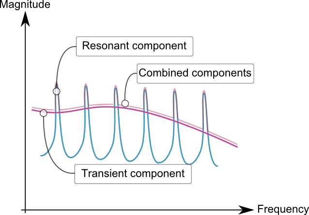
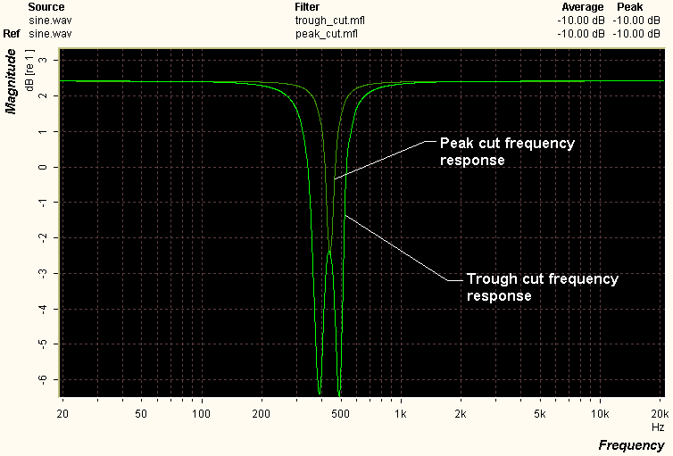
Figure 7: How transient and resonant spectrum components combine to form the average spectrum that Har-Bal sees. The transient component is relatively smooth and spans a wide bandwidth, whilst the resonant component is confined to discrete frequencies. Har-Bal sees the two components combined together.Lets think back to our plucked guitar string example and consider how we might increase the relative amplitude of the transient component over the resonant component. All we need to do to achieve that is to kill the resonance which can easily be achieved by muting the string with a finger. Now think of how a muted guitar string sounds when plucked : a dull thud is an apt description! It may be an extreme example but the conclusion generally holds in the sphere of equalisation, which is that cutting peaks directly tends to a dull lifeless sound. Now lets go back to the generally held belief that you should only apply low Q cutting and boosting and only in moderation. If we consider what happens in this case we see that because of the low Q filtering, any peak modification will have almost the same (but not quite) effect on the content in-between the peaks, thereby not damaging the sound quality much. But now consider the empathetic equalisation approach of cutting a peak by cutting in the adjacent troughs. In this case the greatest cut occurs in the troughs meaning that the resonant content is raised in level relative to the transient content. Thus, with high Q peaking and cutting filtering placed precisely, we can actually make radical changes to the spectrum without bringing about the dullness in sound that often results if trying the same thing using more conventional equalisation equipment. In short, though the low Q filtering recommendation made by mastering engineers does apply to regular equalisation equipment, it does not apply to Har-Bal because Har-Bal has the analysis power to be able to place the boosts and cuts in pricisely the right location to avoid the problems that can result from poorly target equalisation. Here is another contrived example to illustrate this mechanism. We have a 440Hz sine wave mixed with pink noise and propose cutting its level by a nominal 5dB using normal peak cutting and empathetic equalisation trough cutting. The two different filter realisations are illustrated in Figure 8. If we apply these two filter realisations to the pure tone and the pink noise we obtain the results shown in Figures 9 & 10 (in the context of resonant and transient components, the pure tone represents the resonant component and the pink noise represents the transient component). Note that the pure tone spectrum measurement has a noise component mixed in to stop Har-Bal from introducing a large loudness compensation gain change.
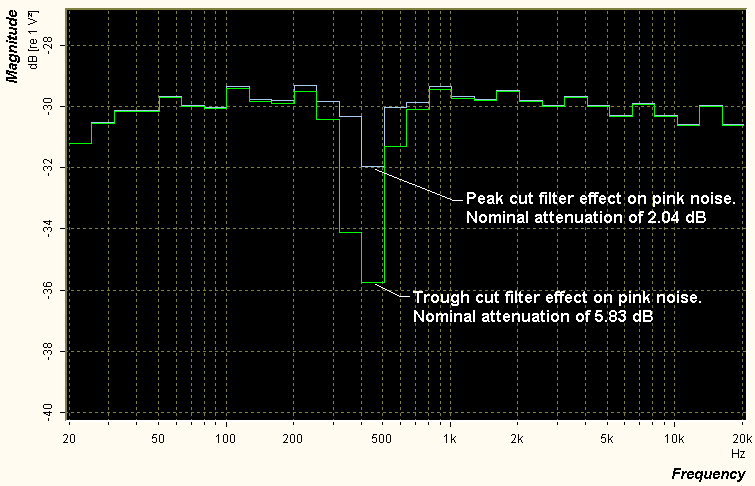
Figure 8: Conventional and Empathetic Equalisation Filter RealisationsIn the pure tone case the 1/3 octave spectrum (measured using a separate spectrum analyser on the Har-Bal filtered wave file) amplitudes of the 440Hz peak are the same, which is what we would logically expect to see. However, in the case of the pink noise the amount of attenuation afforded to the pink noise within that same 1/3 octave band is significantly greater for the Empathetic Equalisation approach (see Figure 9). More importantly we note that in the case of a conventional peak cut filter response the tone is attenuated by 4.74dB whilst the noise in that third octave band is attenuated by only 2.04dB. Thus we have a loss of separation between the noise and the tone of 2.7dB with this filter. In contrast, with the Empathetic Equalisation approach the tone is again attenuated by 4.74dB but in the noise in that third octave band is now attenuated by 5.83dB. Hence we have a increase of separation between the noise and the tone with the Empathetic EQ filter by 1.09dB!
Figure 9: Attenuation of 440Hz Tone by Conventional and Empathetic Equalisation Filter Realisations
Figure 10: Attenuation of Pink Noise by Conventional and Empathetic Equalisation Filter Realisations
Bullet the Blue Sky Continued...Having selected the first section of our partitioned track, lets begin by designing a filter for it. The first thing we should do is switch to 1/3 octave resolution so that we can get a better understanding on where the imbalances in the mix may lie. The importance of 1/3rd octave stems from the tuning of the basilar (the hairs which convert sound to nerve impulses) in human hearing, which approximately corresponds to 1/3rd octave bands (except at that low frequency end where the bands are narrower). 1/3rd octave view therefore gives an impression of the balance that is closely consistent to the way we hear.
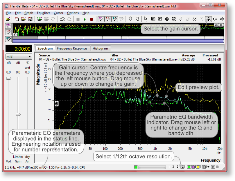
Figure 11: "Bullet the Blue Sky" : the first segment in 1/3rd octave resolutionLooking at the first segment spectrum for "Bullet the Blue Sky" (see Figure 11) in 1/3rd octave resolution, we clearly see areas of weakness and strength over the entire spectrum. There is prominant peaking at 75Hz and 150Hz corresponding to the bass guitar output and prominent peaking at 600Hz and 3kHz corresponding to snare resonance and the lead guitar respectively. There is significant weakness around 300Hz, 1kHz and 7kHz areas. These areas may or may not present auditory problems. The only way to determine if they do is by bringing in more uniformity and seeing if it actually sounds better. The question is, given our hypothesis to test and the empathetic equalisation recommendations on smoothing spectrums, how do we go about achieving this result? Generally speaking, we start by selecting the gain cursor and the 1/12th octave spectrum resoultion and then introduce peaking and cutting at appropriate locations. So how do we do filtering with the gain cursor? The gain cursor is equivalent to a parametric equaliser. The centre frequency is chosen by moving the cursor to the desired frequency on the spectrum plot and then pressing and holding down the left mouse button. The gain is controlled by moving the mouse up or down and the Q is controlled by moving the mouse left or right. During the dragging operation a preview of the filtered spectrum follows the mouse movement. To keep the Q fixed while making boost or cut, hold the SHIFT key down. To keep the Q at the maximum value press and hold the M key down. When you release the left mouse button the filter change is made and the spectrum plots updated. If you wish to cancel an edit press the ESCape key before releasing the left mouse button. The cursor preview is attached to either the peak or the average spectrum plot and you can change the focus from one to the other by pressing the TAB key. Which plot holds focus is shown in the status bar by the focus indicator. The status bar also displays the parametric EQ centre frequency, gain and Q. The values are displayed in scientific notation, which means large and small values are prefixed with the appropriate letter indicating a base 10 multiplier as indicated in Table 2. As an example, 1.1kHz means 1100Hz. Figure 12 Illustrates these aspects of Har-Bal.
Figure 12: Aspects to Performing Parametric EQ Filter Edits
Table 2: Engineering Notation Prefixes and their Corresponding MultipliersContinuing on, we introduce high Q peaking on the peaks and cutting in the troughs in such a way as to smooth out the average spectrum when viewed in 1/3rd octave resolution. We don't alter all peaks and troughs but rather just as much as is necessary to bring a level of smoothness to the spectrum. A point to make in this regard is that the level of smoothing to aim for will depend on the density (in terms of number of instruments) of the recording. If your recording is of a solo instrument great care needs to be taken to not destroy the character of the instrument. With more instruments timbral alteration has much less influence and is generally encouraged (mixing generally involves using EQ to allow different instruments to blend in a more pleasing way) for the sake of allowing each instrument to be heard in a competing landscape. Returning to the process, we smooth by applying edits in 1/12th octave resolution and then checking the 1/3rd octave resolution to see if we are smoothing in the right direction. After a bit of practice you become adept at recognising what is needed in 1/12th octave resolution and rarely need to switch to 1/3rd octave resolution, except for the final check and balance. Using this approach I came up with the following filtered spectrum for the first segment (see Figure 13).
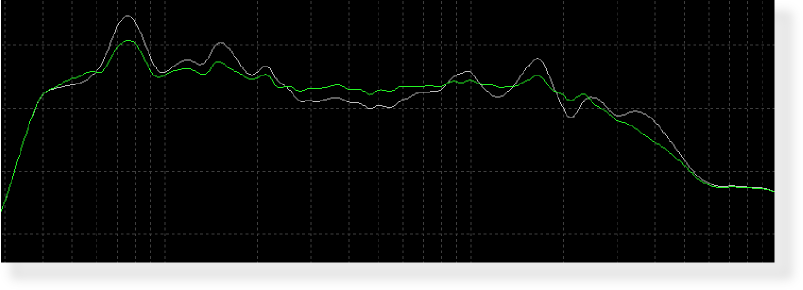
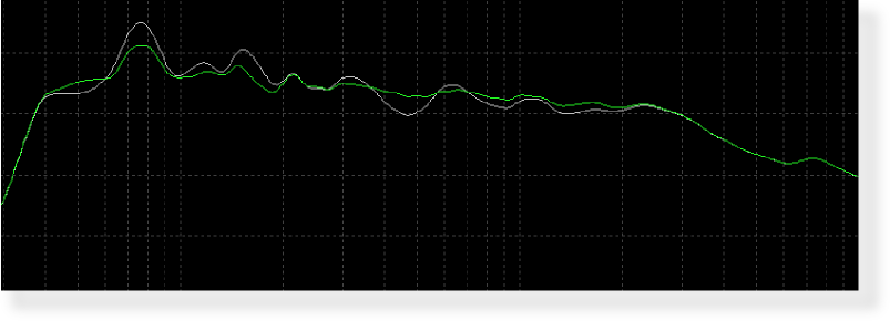
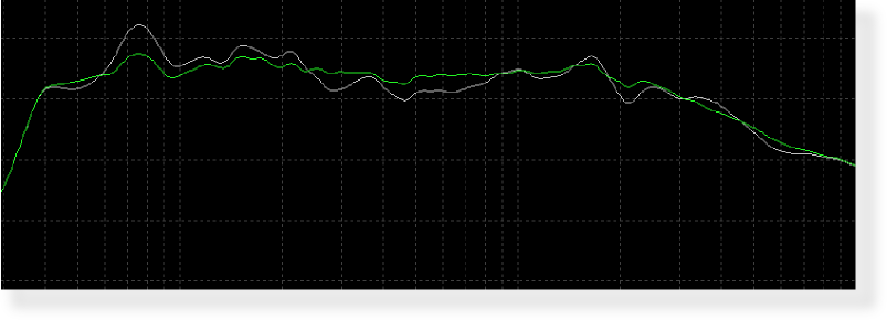
1/3rd Octave Figure 13: Close up of the first segment filtered average spectrum in 1/3rd and 1/12th octave resolution. Note how the filtered spectrum nominally overlays the original to preseve the overall mix intention and cuts are achieved by cutting troughs and boosts are achieved by boosting peaks.The average spectrum is significantly smoother than the original and holds up well on playback. The snare drum shows more definition and the high-hat has extra clarity whilst the bass guitar and kick drum are still prominant parts of the mix. In 1/12th octave resolution you can see how the smoothing has been achieved through selective peaking and cutting. Moving on, we select segment two and apply the same filtering approach to obtain the smoothing results of Figures 14. Likewise, the results of filter designs for segments three through to nine are shown in Figures 15 through 21. Studying these filters, the general approach of smoothing using the empathetic equalisation technique is readily seen. What is readily apparent from this approach and which dramatically sets it apart from other methods of equalisation is the level of detail in the taylored filter frequency responses. It is clear from the 1/12th octave spectrums that to produce a similar response using a hardware equaliser would be difficult, if not impossible.
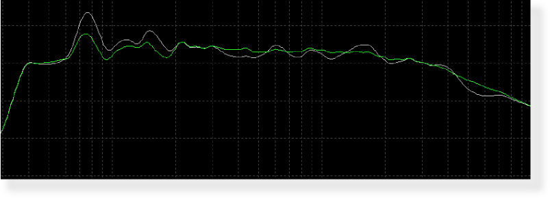
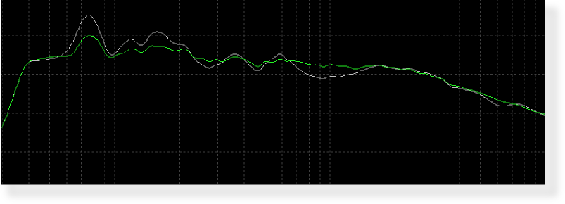
1/3rd Octave Figure 14: Close up of the second segment filtered average spectrum in 1/3rd and 1/12th octave resolution.
1/3rd Octave Figure 15: Close up of the third segment filtered average spectrum in 1/3rd and 1/12th octave resolution.
1/3rd Octave Figure 16: Close up of the fourth segment filtered average spectrum in 1/3rd and 1/12th octave resolution.
1/3rd Octave Figure 17: Close up of the fifth segment filtered average spectrum in 1/3rd and 1/12th octave resolution.
1/3rd Octave Figure 18: Close up of the sixth segment filtered average spectrum in 1/3rd and 1/12th octave resolution.
1/3rd Octave Figure 19: Close up of the seventh segment filtered average spectrum in 1/3rd and 1/12th octave resolution.
1/3rd Octave Figure 20: Close up of the eighth segment filtered average spectrum in 1/3rd and 1/12th octave resolution.
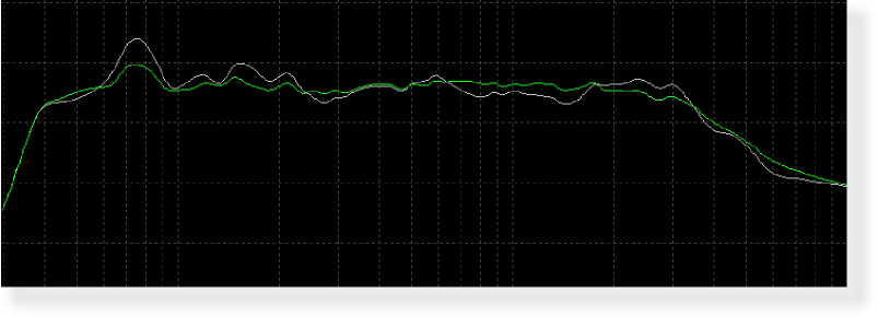
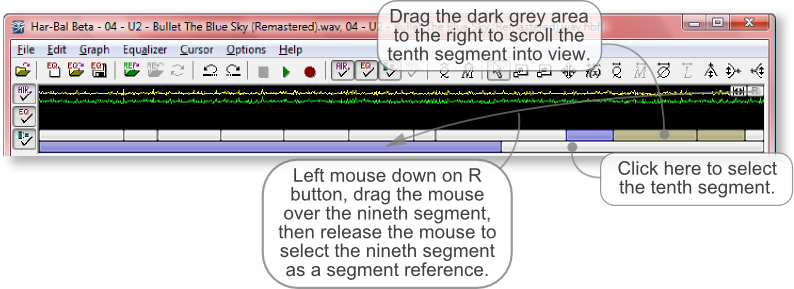
1/3rd Octave Figure 21: Close up of the ninth segment filtered average spectrum in 1/3rd and 1/12th octave resolution.Of the ten segments in our track partitioning, the final one is yet to be addressed. Because the general sparseness of the final segment, the average spectrum is quite irregular and this irregularity can be difficult to interpret. A better way to deal with this segment is to base the segment equalisation upon the segment next to it, the ninth segment. But how to we do this? Segment ReferencingIt is typically common that an equalisation we design for one segment could be applied to another wholesale or with additional of minor customisations. Take for example, the filter we design for a chorus and a track with multiple choruses. It is likely that the ideal response for one chorus will be similiar to another. Likewise, in our case of wanting a seperate filter for the track exit, it is beneficial to be able to base the response on the adjacent segment to avoid having audible tonal discontinuity at the split point. To be able to create filters for other segments based on an existing one, Har-Bal uses a concept called segment referencing. We select a segment as a reference by pressing down the left mouse button down on the "R" button in the time line and dragging the mouse to the segment selector we want as a segment reference and letting go of the mouse button. Then we select the next segment to work on. Figure 22 illustrates how we would do this using the timeline control.
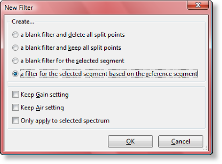
Figure 22: Selecting the ninth segment as segment reference (when the ninth segment is currently selected) and then selecting the tenth segment for editing.Having selected the ninth segment as segment reference and the tenth segment for editing we can create a filter for the tenth segment based on the segment reference using the New Filter menu command. Doing so opens the New Filter dialog box. To copy the reference segment response into the selected segment, select the create... option "a filter for the selected segment based on the reference segment" as shown in Figure 23.
Figure 23: New Filter Dialog Box. Creating a New Filter Based on a Segment Reference.The copied filter response is further modified to give the spectrums shown in Figure 24. Note that because of the sparsity of the instrumentation in the track exit and not wanting to destroy the character of the instruments, the editing is more conservative than in the other segments.
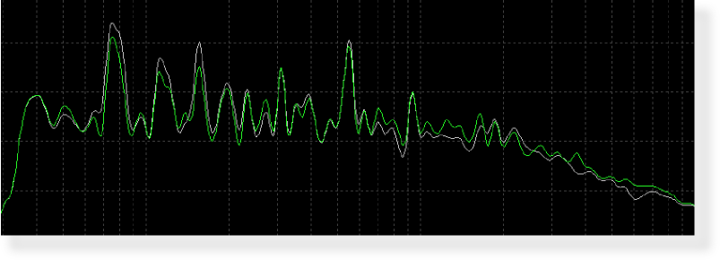
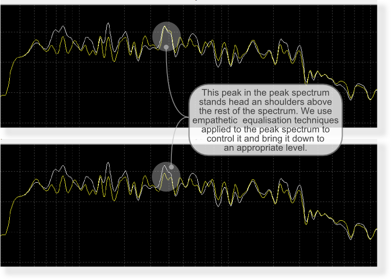
1/3rd Octave Figure 21: Close up of the tenth segment filtered average spectrum in 1/3rd and 1/12th octave resolution.On completing the creation of filters using the empathetic equalisation approach applied to the average spectrum, we need to listen to the track for any disturbing transient material. In particular we should listen and watch out for high peak output at selected frequencies that cause distress. If our processing has created some problem areas then we need to address those. Peak CorrectionIf on listening you hear some distressing output then it can generally easily be tracked down by looking at the peak spectrum in 1/12th octave view. Any stressful transient material will show as a large peak in the peak spectrum trace. As an example the large peak in segment eight of the filter causes audible stress and needs correction (See Figure 22). We do it using the same empathetic equalisation technique as before but now we apply it to the peak spectrum. It is useful to have both the peak and average spectrum traces visible while making this type of adjustment because often the peak and average trends are at odds with one another : correcting the average leads to a large peak in the average and correcting the peaks leads to a large dip in the average. In such cases we have to come to a compromise between the peak and average and we base our decision of judicious listening. In future Har-Bal will have a means of decoupling this problem and tackling peaks on their own but at this point in time "peak taming" is not implemented.
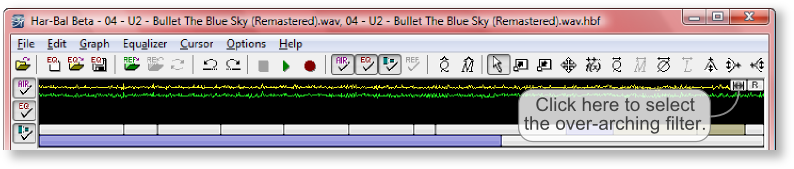
Figure 22: Identify and correct peaks that cause audible distress in the peak spectrum of all segments. Only address a peak if it causes audible distress.The Final StepsHaving corrected the average and peak spectrums we need to re-visit our overall equalisation and see if it is true to the recording. We do so by careful listening and regularly toggling equalisation in and out for the entire track. Doing so reveals that whilst the clarity has been improved we have made the bass subdued and mid-range rather dominant in comparison to the original. Rather than attempt to address this issue by adding extra filter edits to the segment filters there is an easier way. In addition to the segment filters, Har-Bal includes an over-arching filter that combines with the segment filters to create the final outcome. When we need to change the overall balance of the track we use this filter. If you have selected a segment filter but need to now select the over-arching filter all you need do is press the double arrow button in the timeline control as shown in Figure 23.
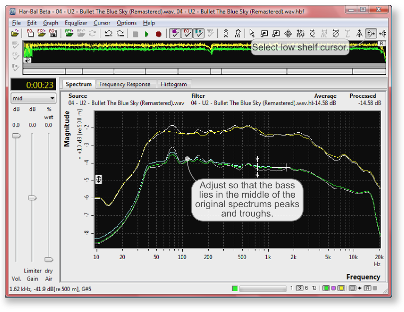
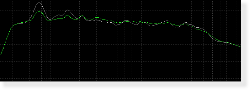
Figure 23: Press the double arrow button to return to the over-arching filter of a segmented filter.Having selected the over-arching filter, it can be seen from the 1/3rd octave resolution average spectrum that the bass region does not nominally overlay the original spectrum but largely lies beneath it, which is why it sounds bass deficient compared with the orginal. However, we do not want to just boost the bass region as it will mask the mid-range so we would like to lift the entire range from about 1.7kHz down to zero so that the weight of the bass end more accurately trends with the original. We can easily do this using the low shelf cursor, as shown in Figure 24. I also introduce a low shelf cut with cutoff frequency of 40Hz to stop the amplification of subsonic content (not shown).
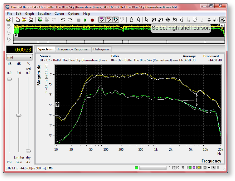
Figure 24: Adjusting the low end balance using the low shelf cursor.Because of the added weight in the mid range that our re-balancing brings, the top end takes on a subdued sound. To address that issue we use the high shelf cursor with a knee at around 3kHz to bring that area more presence (see Figure 25).
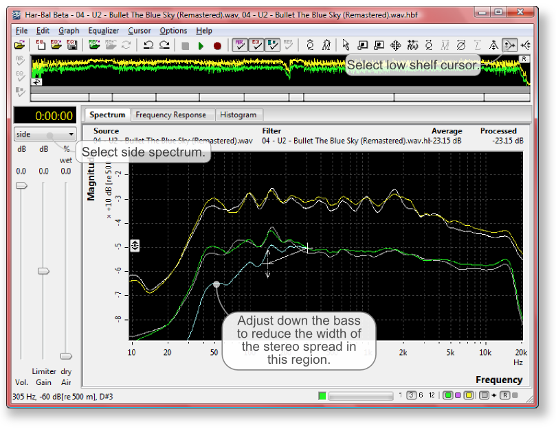
Figure 25: Adjusting the high end balance using the high shelf cursor.Throughout this tutorial so far we have made all our adjustments to the mid spectrum. This is generally the region you will adjust mostly when building filters in Har-Bal. However, occasionally you will also want to introduce modification in the side spectrum to alter the stereo imaging of the track. This track is a good case in point as the bass in this track is quite widely panned. This does not present a big problem when listening through speakers but with the ubiquity of headphone listening in this day and age, wide panned bass sounds quite disturbing. To improve the sound for monitoring in headphones we can modify the side spectrum to bring this change about. By using the low shelf cursor to introduce a cut from 300Hz down we can reduce the panning of the bass parts, producing near mono bass (see Figure 26). To understand how this works consult the Har-Bal introduction.
Figure 26: Reducing the bass stereo spread in the side spectrum using the low shelf cursor.With final listening of the track (particularly when listening through headphones), it is apparent that the track was recorded in a fairly dead recording studio and little ambiance was added during the recording process. This can lead to a sense of detachment from the performance so to add a sense of coherent space to the recording we add 15% air to the recording. Bullet the Blue Sky : Concluding RemarksHaving completed a comprehensive Har-Bal filter for the U2 track Bullet the Blue Sky and hearing the results, it should be patently clear to anyone that harmonic balancing, as applied through Har-Bal, is capable of sonic changes simply not possible via other approaches. The process is complicated but the results are rewarding. The detail required to mimic the process by any other means is simply not possible, owing to the shear number of parameteric equalisation stages required. Now you might think that I am merely eulogising Har-Bal and without a demonstration of this filter that would certainly be the case. So to bring a taste of reality back into this discussion the filter discussed and developed here is freely available from our website (along with filters to a number of other demonstration tracks). Just download the filter and the track and hear for yourself what Har-Bal can do. I appologise whole heartedly to you for having to pay for the track (we don't have a distribution contract with U2 or the other artists) but for less than the price of a good cup of coffee you can be hearing the revelation for yourself. The only caveat I'd place on such a test is to ensure that you download the track from the link provided because a lot of material these days is re-mastered mutliple times so the only way you can be sure of having the same master as the one the filter was developed for, and hence being able to hear the same results, is if you download from the same location. If you happen to have the same track in your CD collection it is tempting to try that version but it may well be a different master, which will undoubtedly give a biased impression of Har-Bal.
More on the Har-Bal Timeline
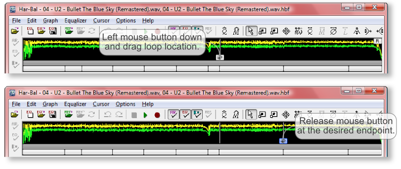
Playback Navigation and LoopingNavigating playback to a particular point in the track is as simple as clicking on the desired location in the time line. You can also do this during playback. The starting location of playback is the selected location in the time line. This location is returned to when playback is stopped unless the "return to start when play stopped" option in the Har-Bal Preferences dialog is not checked. When not checked, playback continues from the last position reached. If the option is checked and the playback position is changed while playing the start position does not change. It only changes if the change is made when not in playback. Looping is achieved by setting up a looping interval before pressing play. The start of the loop is the starting location for playback and the end of a loop is set by dragging the looping button to the desired location (see Figure 27). A loop can be cleared by dragging the looping position to a time in the time line before the start time. During playback the loop end time can be altered.
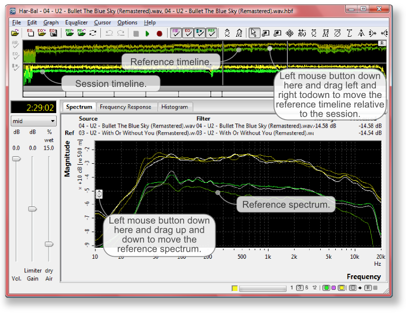
Figure 27: Setting playback loops.Playable ReferencesWith the Open Reference command you can open a sound file to use as an audible reference which you can toggle in and out of playback as an aid to building compilations with a consistent tone. Note that for a sound file to be a "playable" reference it must have the same sample rate as the session sound file. If they differ the toggle reference option will be greyed out.
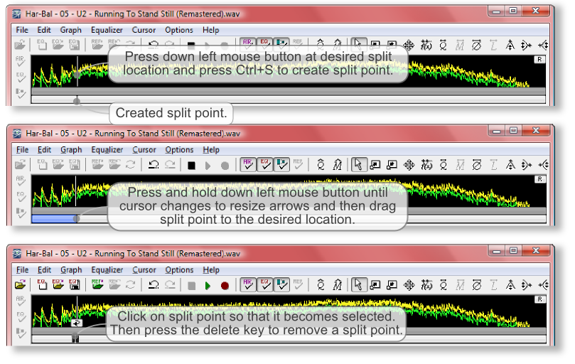
Figure 28: Playable references.When a playable reference is opened the timeline for the referene is displayed above the timeline for the session and the spectrum for the reference displayed in the spectrum view (see Figure 28). The reference timeline can be dragged horizontally relative to the session timeline so that any part of the reference can be played in sync with any part of the session. Similarly, the reference spectrum can be dragged vertically to align with the session spectrum as an aid to understanding and correcting for differences in tonality. Creating, Deleting and Moving Split PointsSplit points are created by pressing and holding down the left mouse button at the location of the split on the timeline and then pressing Ctrl+S on the keyboard. The best way to determine the split location is by playing the track and clicking on the start location. When you release the left mouse button playback will resume from that location and through listening we can easily hear if the location captures the content we want in a segment. If it doesn't then we reposition and try again. When we have found the correct location we press and hold in the left mouse button and press Ctrl+S on the keyboard to create the split. If the split location needs adjusting we can do so by pressing the left mouse button down while over the split marker and waiting for the cursor to change to horizontal a resize cursor. When it has we can then drag the split point left or right of its current position and release the left mouse button to establish the new position. To delete a split point we click on the split marker to select it. Then once selected simply press the delete key on the keyboard to delete the split point. These different scenarios are illustrated in Figure 29.
Figure 29: Creating, Deleting and Moving Split Points.
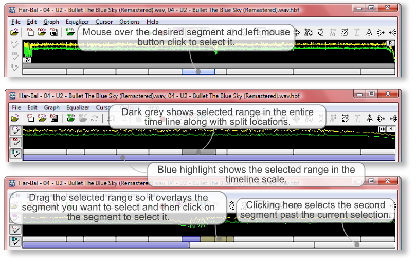
Selecting and Navigating SegmentsWhen in full timeline view you select a segment by mousing over the desired segment in the top bar and left mouse button clicking (see Figure 30). When a a segment is already selected you do not need to return to full timeline view to select a new segment. An easier way is to drag the selected range in the top bar so that it overlays the segment you would like to select and then click on the segment in the bottom bar to change the selection to it.
Figure 30: Navigating Segments.Concluding RemarksThis tutorial is by no means extensive. For the sake of getting you up and running we have deliberately left it as a shortish introduction of what we think you should know. There is much more that we could discuss but for the sake of brevity we have left that untouched. If you haven't already done so you can find extra details on the workings of Har-Bal and some of the new functionality in the introduction, and a discussion of the concept of loudness compensation here. For the features untouched in this tutorial, you can easily find help using the help system in Har-Bal. To use the help system consult the instructions found here. Finally, the Har-Bal forum has a wealth of information on it regarding much of what has been left out of this tutorial. I encourage you to make use of it. |

 1/12th Octave
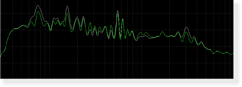
 1/12th Octave
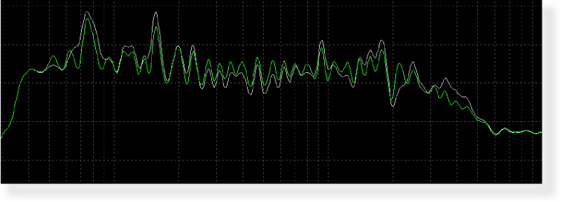
 1/12th Octave
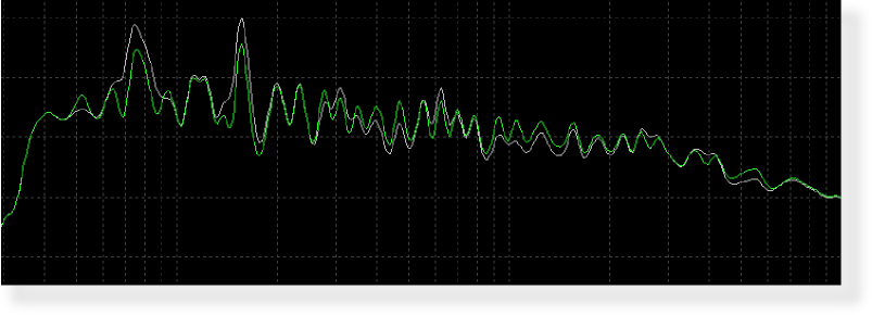
 1/12th Octave
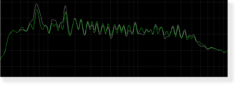
 1/12th Octave
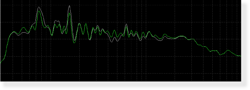
 1/12th Octave
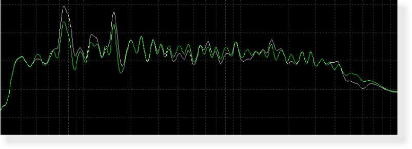
 1/12th Octave
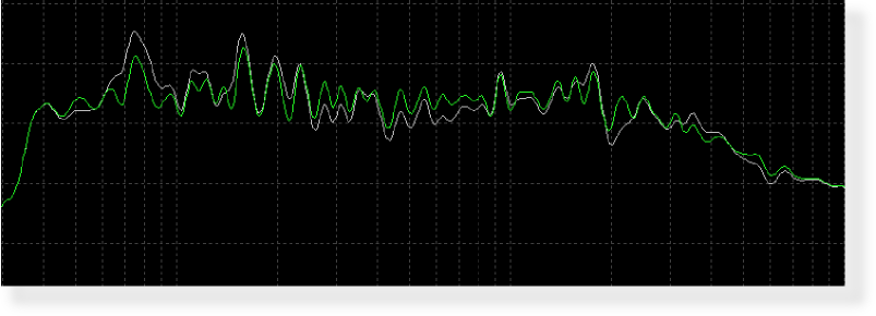
 1/12th Octave
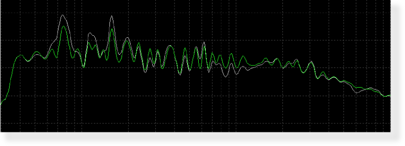
 1/12th Octave
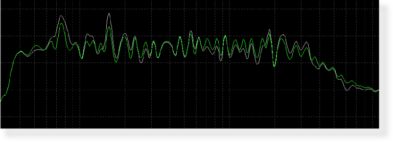
 1/12th Octave